# Setup
%matplotlib inline
import numpy as np
import matplotlib.pyplot as plt
import matplotlib
params = {'font.size'     : 14,
          'figure.figsize':(10.0, 6.0),
          'lines.linewidth': 2.,
          'lines.markersize': 8,}
matplotlib.rcParams.update(params)

Optimization¶

Scope¶

Mathematical optimization aims at solving various kinds of problems by minimizing a function of the form:

\[f(X) = e\]

Where \(f\) if the cost function, \(X\) is a \(N\) dimensional vector of parameters and \(e \in \mathscr R\). More informations about the underlying theory, the nature of the solution(s) and practical considerations can be found:

On Wikipedia,
On (excellent) Scipy lectures.

Solving¶

Scipy offers multiple approaches in order to solve optimization problems in its sub package optimize

General purpose approach¶

scipy.optimize.minimize allows one to use multiple general purpose optimization algorithms.

from scipy import optimize

def f(X):
  """
  Cost function.
  """
  return (X**2).sum()

X0 = [1.,1.] # Initial guess
sol = optimize.minimize(f, X0, method = "nelder-mead")
X = sol.x
print "Solution: ", X

Solution:  [ -2.10235293e-05   2.54845649e-05]

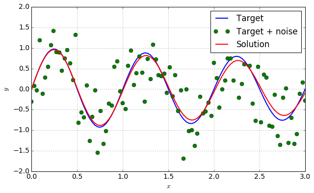
Curve fitting using least squares¶

In order to perform curve fitting in a more convenient way, scipy.optimize.curve_fit can be used.

def func(x, omega, tau):
    return np.exp(-x / tau) * np.sin(omega * x)


xdata = np.linspace(0, 3., 100)
y = func(xdata, omega = 2. * np.pi, tau = 10.)
ydata = y + .5 *  np.random.normal(size=len(xdata))

params, cov = optimize.curve_fit(func, xdata, ydata)
omega, tau  = params
ysol = func(xdata, omega, tau)


fig = plt.figure(0)
plt.clf()
plt.plot(xdata, y, label = "Target")
plt.plot(xdata, ydata, "o", label = "Target + noise")
plt.plot(xdata, ysol, label = "Solution")
plt.grid()
plt.xlabel("$x$")
plt.ylabel("$y$")
plt.legend()
plt.show()